PSIRpicker Tutorial
1. Introduction to PSIRpicker
P and S arrival times are fundamental information of seismic events. In seismology research, we usually have acess to earthquake catalogs provided by government agency or regional seismic networks (e.g., USGS, SCSN). However, these catalogs generally have no phase arrival information for stations that are not rountinely used for earthquake locations. As a result, picking P/S arrivals is necessary. There are two ways to do it automatically:
1) use a velocity model and catalogued event location to predict arrivals;
2) use detector functions (e.g., STA/LTA) to pick sharp amplitude change.
As the velocity model may not be accurate, the first approach is usually not satisfactory. Using a detector function is also not optimal, because the performance of detector functions tends to decrease in presence of high-amplitude local noise or seismic phases other than the targeted phases.
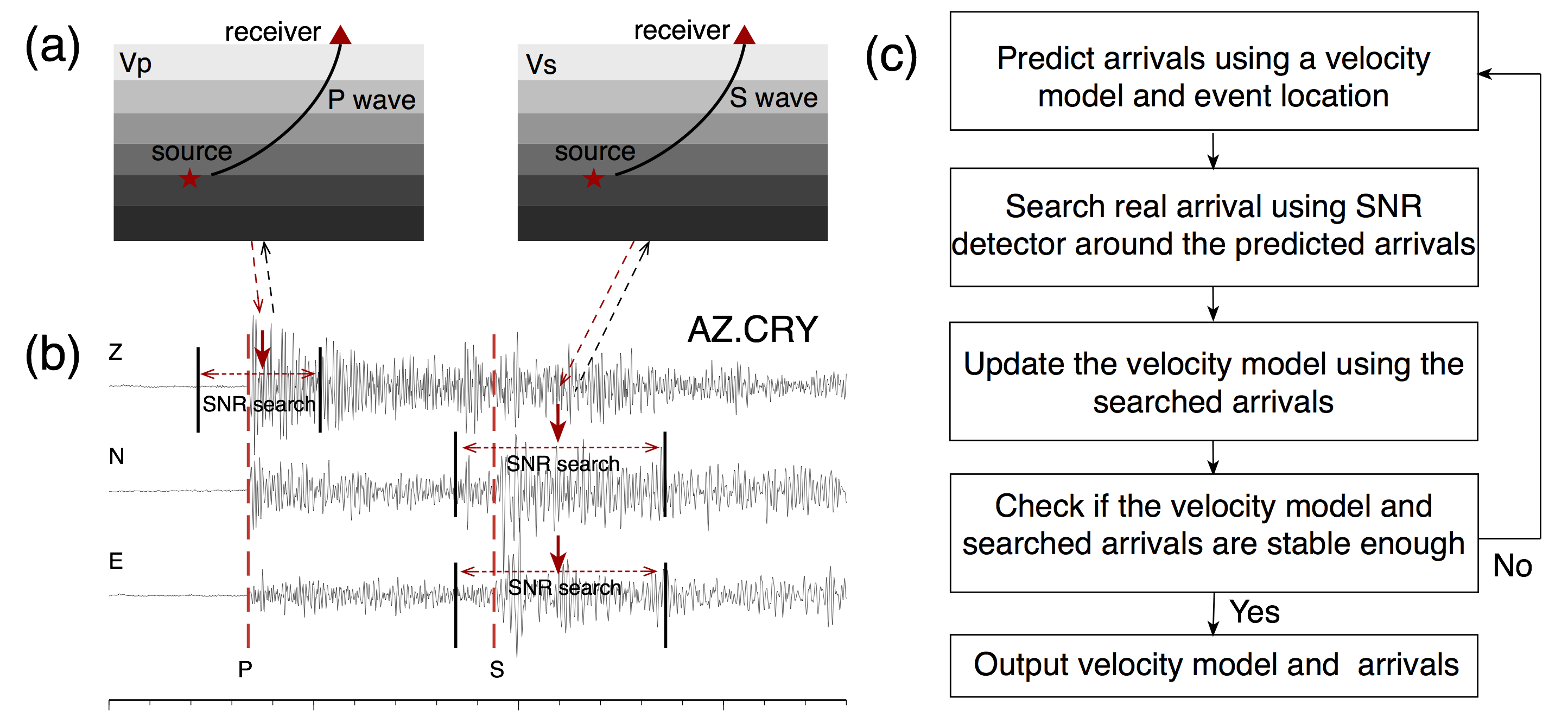
PSIRpicker (Li and Peng, 2016) provides a simple way to combine both methods, in order to obtain better accuracy and higher pick production than each alone. Our algorithm is briefed as "Predict-Search-Invert-Repeat" (PSIR), with details outlined below (also in Fig. 1):
1) Predict initial picks using an initial velocity model;
2) Search genuine phase arrivals around the predicted ones using a detector function;
3) Invert the velocity model using the searched picks;
4) Predict new arrivals using the inverted velocity model;
5) Repeat 1) ~ 4) until the picks and velocity model become stable.
Primary advantages of this method include:
1) Avoid picks clearly outside typical P/S arrival windows;
2) Iteratively update the velocity model to increase prediction accuracy. The derived velocity model could be used for further study purposes.
2. Code setup
PSIRpicker is written in Matlab. An auxiliary package, MatSAC, is required to read SAC files. The code calls a few Matlab built-in functions, and is running without any problems with the 2012 version or later. Some of built-in functions (such as strsplit) may be missing in older Matlab versions, but hopefully you could find substitutes on the internet.
For internal GT users, the simplest way is to add the package path into your matlab path, i.e., add the following line in your ~/.bashrc:
export MATLABPATH="/home/zli/matlab/PSIRpicker:/home/zli/matlab/MatSAC:$MATLABPATH"
For outside users, please download PSIRpicker and MatSAC first, put them in your own directory and add the paths to MATLABPATH. For example, in bash prompt, type:
tar -xzvf PSIRpicker_v1.0.tar.gz
tar -xzvf MatSAC.tar.gz
mkdir ~/matlab
mv PSIRpicker ~/matlab/
mv MatSAC ~/matlab/
Then add the following line in your ~/.bashrc:
export MATLABPATH="~/matlab/PSIRpicker:~/matlab/MatSAC:$MATLABPATH"For either GT or outside users, do not forget to make it effective right away in bash prompt:
source ~/.bashrc
If done correctly, launch Matlab and type in the command window:
help PSIRpicker
Then you should see the full usage information about PSIRpicker.
3. Prepare input files
Data files:The code reads SAC files. Event occurrence time should be written in kztime, and o time should be shifted to zero. Other SAC headers that need to be written include evlo, evla, evdp, stlo, stla, stel. Note that stel should be in meter, while evdp in kilometer. These headers are of much importance; any lost information will lead to incorrect results.
Meta files:Three input files include event.cat, vp0.dat, vs0.dat.
event.cat contains the data entries (format: station_name event_id E_component N_component Z_component). Example:
CRY 20120104230605 /data4/sjfz/zli/anisotropy/data/FZ/CRY/20120104230605.CRY.e /data4/sjfz/zli/anisotropy/data/FZ/CRY/20120104230605.CRY.n /data4/sjfz/zli/anisotropy/data/FZ/CRY/20120104230605.CRY.z
CRY 20120105021430 /data4/sjfz/zli/anisotropy/data/FZ/CRY/20120105021430.CRY.e /data4/sjfz/zli/anisotropy/data/FZ/CRY/20120105021430.CRY.n /data4/sjfz/zli/anisotropy/data/FZ/CRY/20120105021430.CRY.z
CRY 20120109122413 /data4/sjfz/zli/anisotropy/data/FZ/CRY/20120109122413.CRY.e /data4/sjfz/zli/anisotropy/data/FZ/CRY/20120109122413.CRY.n /data4/sjfz/zli/anisotropy/data/FZ/CRY/20120109122413.CRY.z
Note the file paths could be absolute or relative to the work directory. For each entry, all three components should be placed in the same line (in the above example, web browser may display them in separate lines due to wrapping control).
vp0.dat and vs0.dat contain initial P and S velocity models, respectively (format: velocity, upper_boundary_depth).
vp0.dat example:
5.9535 0
6.0636 5
6.2308 10
6.2962 15
6.3724 20
6.6576 25
7.7365 30
vs0.dat example:
3.4056 0
3.5602 5
3.6995 10
3.7116 15
3.5399 20
3.7881 25
4.5247 30
GT users can copy event.cat vp0.dat vs0.dat from /home/zli/PSIRpicker_example to your own directory. The SAC files in the example are stored in /data4/sjfz/zli/anisotropy/data/FZ/CRY/. Note that in this case I put only one station. In practice you can include multilple stations in a single run, as long as they are listed in event.cat.
Outside users can download the sample data and input files here, in which I also included my test outputs for your reference.
4. Run PSIRpicker
Using PSIRpicker is straightforward. Open Matlab in the directoy where you place the meta files (event.cat, vp0.dat, vs0.dat). First type in Matlab command line:
PSIRpicker(0)
This mode uses the initial velocity models in vp0.dat vs0.dat to predict initial P and S arrivals. The searched picks are stored in pick.dat, and updated velocity models are stored in vp.dat vs.dat. Then type:
PSIRpicker(1)
Different from the first step, this mode uses the updated velocity models in vp.dat vs.dat produced previously. By runing this, pick.dat and vp.dat vs.dat will be updated again.
Likewise, you can type:
PSIRpicker(n)where n is a user-defined integer to keep track of your run step. It updates the picks (stored in pick.dat) and velocity models (stored in vp.dat and vs.dat) based on the velocity models obtained in the latest step.
5. Check output files
The code produces several output files:
- pick.dat: arrivals and SNRs of p and s picks.
format: station_name, event_id, p_arrival, p_snr, s_weigthed_arrival, s_average_snr, s_arrival_e_component, s_snr_e_component, s_arrival_n_component s_snr_n_component.
Recordings that failed to be picked are tagged with SNR<0. Final S arrival is SNR-weighted average of picks on E and N components. - vp.dat, vs.dat: updated P and S velocity models.
- hist_p.ps, hist_s.ps: histograms of residuals between searched picks and predicted picks during that run, for P and S, respectively.
- ptime.dat, stime.dat: contain matrixes used for velocity inversion.
6. Advanced usages
PSIRpicker takes up to three arguments. Full usage can be found by Matlab help.The first one is velocity model used to compute theoretical arrivals. In addition to the example in Part 4, setting first argument to -1 calls a built-in 1D velocity model from southern California. Note that in this case vp0.dat vs0.dat are not required. By running default models, files storing updated velocity models are created (vp.dat, vs.dat). So you can use positive run step tracker (1~n) afterwards.
PSIRpicker(-1); % run with built-in velocity models.The second argument is the maximum allowed velocity perturbation, which is to determine the search window around the predicted arrival. For example, if the initial velocity model is very crude, a wider search window is preferred in order to capture genuine arrivals. If the initial velocity model is precise enough, a narrow window would reduce picks at unwanted phases. A default value of velocity perturbation is 10%. If initial velocity models are bad, one can use 20% or 30% at first, then reduce it in the later runs as velocity models are improved gradually.
PSIRpicker(0, 0.2); % run with initial models and allow 20% velocity perturbation.The third argument is the window length used to calculate SNR function, which is related to a tradeoff between pick sharpness and stablenss. Longer window produces more stable result, while compromises temporal resolution and sometimes cannot pick very sharply at the first break. The empirical rule is: long window for noisy data, and short window for clean data. Window to search S wave is typically longer than that for P wave, because S wave suffers from P wave code. Default values are 0.2s for P and 0.4s for S.
PSIRpicker(0, 0.1, [0.1 0.2]); % run with initial models and allow 10% velocity perturbation, use 0.1s for searching P and use 0.2s for searching S.
7. Further notes
- The code does not write the picks into SAC files. However, it is a good practice to write the picks in the SAC files to check overall accuracy.
- The code does not handle event depths shallower than the station elevation. An error would be reported in this case.
- If errors occur, first check if all required SAC headers are written and times are properly shifted.
- A large number of event-station pairs is necessary for obtaining a robust velocity model update. That is, the updated model is not reliable if only tens of event-station pairs are used.
- Questions/comments are directed to zli354 AT gatech DOT edu.
- Please cite the reference below if your work ends up with publication:
Li, Z. and Z. Peng, 2016, An automatic phase picker for local earthquakes with predetermined locations: Combining a signal-to-noise ratio detector with 1D velocity model inversion, Seismol. Res. Lett.., 87(6), 1397-1405.
8. Update notice
- A bug in inv1d.m is fixed. Re-downloading the package is recommended. Thu Jan 5 17:17:03 EST 2017.
Last updated by Zefeng Li at Georgia Tech, Thu Jan 5 17:17:51 EST 2017