Introduction to Travel Time Calculation

by Zhigang Peng

This website contains a brief tutorial on how to compute travel times based on 1D velocity models and existing software packages. This is part of the lecture course titled "Seismology II" offered to the Geophysics graduate students at GT in Spring 2008 by Professor Zhigang Peng .

Part I: TauP Package

Overview of the TauP Toolkit
How to run it at GT geophysics laboratory
Tools included with the TauP package
Phase naming in TauP
Examples
Part 2: COMPLOC Earthquake Location Package
Overview of the COMPLOC Package
Example of a 1D "layered cake" velocity model
Resample the velocity model
Compute the travel time table
Compute travel time for individual SAC traces
Part 3: Write your own travel time calculator
Usin the LAYERXT code in Shearer (1999) book

Overview of the TauP Toolkit

The TauP Toolkit is a seismic travel time calculator developed by seismologists at University of Southern Carolina (SC) [not USC trojan ].
In addition to travel times, it can calculate derivative information such as ray paths through the earth, pierce and turning points.
It handles many types of velocity models and can calculate times for virtually any seismic phase with a phase parser.
It is written in Java so it should run on any Java enabled platform.
Unfortunately, this also means that it is running a little bit slower than other programs. 8-(
The latest version, 1.1.7 can be downloaded at http://www.seis.sc.edu/TauP/ .
Online manual can be viewed at http://www.seis.sc.edu/downloads/TauP/taup.pdf .

How to run it at GT geophysics laboratory

TauP is already installed at "/usr/local/geophysics/TauP". To run it, please add the following two lines in your .bashrc file.
```
export TAUP_HOME=/usr/local/geophysics/TauP
export PATH=${TAUP_HOME}/bin:$PATH
```
After that, type
```
% source ~/.bashrc
% taup_time -help
```
If you get a help output for the taup_time, it is working. 8-)

Tools included with the TauP package

	Name	Brief Description
	taup_time	calculate travel times.
	taup_pierce	calculates pierce points at model discontinuities and specified depths.
	taup_path	calculates ray paths, depth versus epicentral distance.
	taup	a GUI that incorporates the time, pierce and path tools. This requires swing, and hence may not work on some java1.1 systems.
	taup_table	outputs travel times for a range of depths and distances in an ASCII file
	taup_setsac	puts theoretical arrival times into sac header variables.
	taup_create	creates a .taup model from a velocity model.
	taup_create	creates a .taup model from a velocity model.
	taup_peek	peeks at a saved model, useful only for debugging.

Phase naming in TauP

Examples

Compute travel times for S and P for a 200 kilometer deep source at a distance of 57.4 degrees.

22.> taup_time -mod prem -h 200 -ph S,P -deg 57.4

Model: prem
Distance   Depth   Phase   Travel    Ray Param   Purist    Purist
  (deg)     (km)   Name    Time (s)  p (s/deg)  Distance   Name
----------------------------------------------------------------
   57.40   200.0   P        566.77     6.968      57.40  = P    
   57.40   200.0   S       1028.60    13.018      57.40  = S

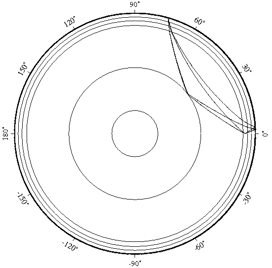
taup_path takes a .taup file generated by TauP Create and generates the path that the phases travel. The output is in GMT (Wessel and Smith, 1995) “psxy” format, and is placed into the file “taup path.gmt”. If you specify the “-gmt” flag then this is a complete script with the appropriate “psxy” command prepended, so if you have GMT installed, you can just:
```
27.> taup_path -mod iasp91 -h 550 -deg 74 -ph S,ScS,sS,sScS -gmt
28.> ls *.gmt
taup_path.gmt
29.> sh taup_path.gmt
30.> gs taup_path.ps
```
If we want to see the travel time curves for these phases, we can do that using taup curve. It works very similarly to taup path except that we don’t need to specify a distance.
```
55.> taup_curve -mod prem -h 143.2 -ph P,S,PcP,ScS,SKS,sS,SS,PKKP -o premCurves.gmt -gmt
56.> sh premCurves.gmt
57.> gs premCurves.ps
```
More examples can be found at the TauP online manual .

Part II: COMPLOC Earthquake Location Package

Overview of the COMPLOC Package

COMPLOC is a Fortran77 computer program package for relocating earthquakes using the source-specific station term (SSST) method.
The source code is available at http://igpphome.ucsd.edu/~glin/COMPLOC/
The related reference is: Lin, G. and P. Shearer (2006), The COMPLOC earthquake location package, Seism. Res. Lett., 77, 440-444.

The entire package are installed in /usr/local/geophysics/COMPLOC_1.01.

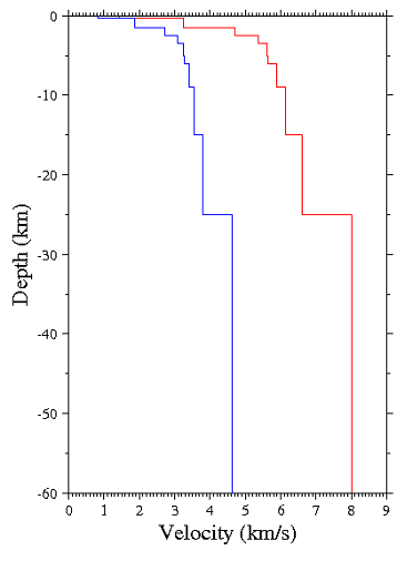
Example of a 1D "layered cake" velocity model

Let's start with a 1D 'layered cake' velocity model, which is pretty much the same form the NCSN used for routine earthquake location.

# Dep Vp (km/s) Vs (km/s)
 0.00    1.42    0.82
 0.25    1.42    0.82
 0.25    3.24    1.87
 1.50    3.24    1.87
 1.50    4.72    2.73
 2.50    4.72    2.73
 2.50    5.36    3.09
 3.50    5.36    3.09
 3.50    5.60    3.23
 5.00    5.60    3.23
 5.00    5.65    3.26
 6.00    5.65    3.26
 6.00    5.90    3.41
 9.00    5.90    3.41
 9.00    6.15    3.55
15.00    6.15    3.55
15.00    6.60    3.81
25.00    6.60    3.81
25.00    8.00    4.62
100.0    8.00    4.62

Resample the velocity model

We can resample the velocity model using "vzfillin" program in the COMPLOC package.
vzfillin.f is a utility program that reads (z, vp, vs) model files and resamples them at any desired finer depth interval. This is done with linear interpolation of parameters between depth points so that models with velocity gradients are easily included.
Here we use the 'layered cake' model above, and do not interpolate the parameters between depth points. So the vzfillin program only fill with constant values between different depth intervals.
Please start by creating a file named 'vz.PKD.layercake'. You can directly download it from this link , or copy and paste the value from the previous window (without the comment).
Then download this parameter file vz.PKD.in , and run the following command:
```
73.> vzfillin < vz.PKD.in
```

Or, you can directly run the command like this:

75.> vzfillin
 Enter input model file name
vz.PKD.layercake
 Enter output file name
vz.PKD.layercake.1km
 Enter Vp/Vs ratio if Vs=0 in input (e.g., 1.732)
1.732
 Enter output dz spacing (e.g. 1)
1

The output is the resampled velocity model vz.PKD.layercake.1km with 1 km depth interval.

Compute the travel time table

The next step is to compute a travel time table, based on the resampled velocity model. Please download the input parameter pkd.p.in , then use the "deptable" program.
deptable.f is a f77 program that computes tables of travel time, ray angle, ray parameter, and vertical slowness at the source as a function of source depth and source-receiver distance.

Please use the following command line:

77.> deptable < pkd.p.in
 Enter input velocity model
 First column of input:  1=depth, 2=radius
 finished reading model
 Depth points in model=  115
 ************************* Table of Model Interfaces **********************
  Depth  Top Velocities  Bot Velocities    -----Flat Earth Slownesses-----
              vp1  vs1        vp2  vs2       p1      p2        s1      s2
   0.2    1  1.42 0.82    2  1.42 0.82   0.70423 0.70420   1.21951 1.21946
   0.2    2  1.42 0.82    3  3.24 1.87   0.70420 0.30863   1.21946 0.53474
   1.5    5  3.24 1.87    6  4.72 2.73   0.30857 0.21181   0.53463 0.36621
   2.5    8  4.72 2.73    9  5.36 3.09   0.21178 0.18649   0.36616 0.32350
   3.5   11  5.36 3.09   12  5.60 3.23   0.18646 0.17847   0.32345 0.30943
   5.0   14  5.60 3.23   15  5.65 3.26   0.17843 0.17685   0.30935 0.30651
   6.0   16  5.65 3.26   17  5.90 3.41   0.17682 0.16933   0.30646 0.29298
   9.0   20  5.90 3.41   21  6.15 3.55   0.16925 0.16237   0.29284 0.28129
  15.0   27  6.15 3.55   28  6.60 3.81   0.16222 0.15116   0.28103 0.26185
  25.0   38  6.60 3.81   39  8.00 4.62   0.15092 0.12451   0.26144 0.21560
 100.0  114  8.00 4.62  115  8.00 4.62   0.12304 0.12304   0.21305 0.21305
 Enter maximum depth (9999 for none)
 Source depths:  (1) Range, (2) Exact
 Enter source dep1,dep2,dep3 (km)
 (1) P-waves  or  (2) S-waves
 pmin, pmax =   0.  0.704225361
 Enter number of rays to compute
 Enter min p at long range (.133 = no Pn, .238 = Sn)
 Completed ray tracing loop
 (1) del in km, t in sec  or  (2) del in deg., t in min
 Enter output file for ray table (or none)
 Enter del1,del2,del3 (min, max, spacing)
 ***Warning: p>u in angle calculation
    Ray assumed horizontal
  0.  0.  0.  0.704228759  0.704225361
 Enter output file name for travel times
 Enter output file name for source ray angles
 Enter output file name for ray parameters
 Enter output file name for vertical slowness at source

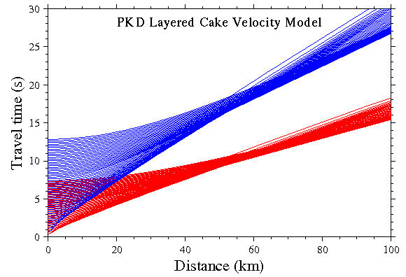
You will get a travel time table PKD.tt.P (plus other tables) that lists the arrival time for different combinations of depth and range (distance).
You can use the following GMT script gmt.PKD.ttime to plot the travel time table. The output will look like this:
For detailed information about each parameters, please read online version of reloc.lin.man_1.0 , or from the following local directory: /usr/local/geophysics/COMPLOC_1.01/reloc.lin.man_1.0

Compute travel time for individual SAC traces

Finally, you can use a program named "gentt" written by me to compute the travel time for P and S waves based on the event longitude, latitude and depth (evlo, evla, evdp), and station longitude and latitude (stlo, stla). This program can be used together with the "saclst" program. See the previous SAC Tutorial for more details about how to use "saclst".

Please download the following tar file for event 20040930043645 (one of the SAFOD targeting event) recorded by the HRSN borehole network at Parkfield, CA, and untar it:

49.> wget http://geophysics.eas.gatech.edu/people/zpeng/Teaching/EAS8803_S08/ttime/HRSN_20040930043645_BP1.tar.gz
# download the tar.gz file
50.> tar zxvf HRSN_20040930043645_BP1.tar.gz
# untar the file
51.> saclst stlo stla evlo evla evdp o a t0 f *BP1*.SAC
BP.CCRB.BP1.SAC    -120.5516     35.9572   -120.5433     35.9867      2.5640      0.0000 -12345.0000 -12345.0000
BP.EADB.BP1.SAC    -120.4226     35.8952   -120.5433     35.9867      2.5640      0.0000 -12345.0000 -12345.0000
BP.FROB.BP1.SAC    -120.4869     35.9109   -120.5433     35.9867      2.5640      0.0000 -12345.0000 -12345.0000
BP.GHIB.BP1.SAC    -120.3473     35.8322   -120.5433     35.9867      2.5640      0.0000 -12345.0000 -12345.0000
BP.JCNB.BP1.SAC    -120.4311     35.9390   -120.5433     35.9867      2.5640      0.0000 -12345.0000 -12345.0000
BP.JCSB.BP1.SAC    -120.4340     35.9212   -120.5433     35.9867      2.5640      0.0000 -12345.0000 -12345.0000
BP.LCCB.BP1.SAC    -120.5142     35.9801   -120.5433     35.9867      2.5640      0.0000 -12345.0000 -12345.0000
BP.MMNB.BP1.SAC    -120.4960     35.9565   -120.5433     35.9867      2.5640      0.0000 -12345.0000 -12345.0000
BP.RMNB.BP1.SAC    -120.4777     36.0009   -120.5433     35.9867      2.5640      0.0000 -12345.0000 -12345.0000
BP.SCYB.BP1.SAC    -120.5366     36.0094   -120.5433     35.9867      2.5640      0.0000 -12345.0000 -12345.0000
BP.VARB.BP1.SAC    -120.4471     35.9261   -120.5433     35.9867      2.5640      0.0000 -12345.0000 -12345.0000
BP.VCAB.BP1.SAC    -120.5339     35.9216   -120.5433     35.9867      2.5640      0.0000 -12345.0000 -12345.0000
# waveform name     stlo         stla       evlo          evla        evdp           o        a          t0
#                 station        station    event         event       event       origin    P wave      S wave
#                 longitude      latitude  longitude      latitude    depth        time   arrival time arrival time

# list the various sac header that will be used as the input for the "gentt" program.

52.> saclst stlo stla evlo evla evdp o a t0 f *BP1*.SAC | gentt -r 1.732 -t PKD.tt.P
BP.CCRB.BP1.SAC      3.35780      2.56400      0.00000 -12345.00000 -12345.00000      1.20479      2.08670
BP.EADB.BP1.SAC     14.88933      2.56400      0.00000 -12345.00000 -12345.00000      3.36663      5.83100
BP.FROB.BP1.SAC      9.83005      2.56400      0.00000 -12345.00000 -12345.00000      2.43450      4.21655
BP.GHIB.BP1.SAC     24.63575      2.56400      0.00000 -12345.00000 -12345.00000      5.11355      8.85667
BP.JCNB.BP1.SAC     11.42158      2.56400      0.00000 -12345.00000 -12345.00000      2.73095      4.73001
BP.JCSB.BP1.SAC     12.24973      2.56400      0.00000 -12345.00000 -12345.00000      2.88469      4.99629
BP.LCCB.BP1.SAC      2.72452      2.56400      0.00000 -12345.00000 -12345.00000      1.09062      1.88896
BP.MMNB.BP1.SAC      5.42452      2.56400      0.00000 -12345.00000 -12345.00000      1.60061      2.77225
BP.RMNB.BP1.SAC      6.12150      2.56400      0.00000 -12345.00000 -12345.00000      1.73660      3.00779
BP.SCYB.BP1.SAC      2.59038      2.56400      0.00000 -12345.00000 -12345.00000      1.06761      1.84910
BP.VARB.BP1.SAC     10.97861      2.56400      0.00000 -12345.00000 -12345.00000      2.64844      4.58710
BP.VCAB.BP1.SAC      7.27293      2.56400      0.00000 -12345.00000 -12345.00000      1.95868      3.39243
# waveform name      dist         evdp          o         a_old       t0_old      a_computed   t0_computed
#                  range (km)     event        origin   old P wave  old S wave  Computed P wave Computed S wave
#                                 depth        time    arrival time arrival time     arrival time arrival time

# compute the P and S wave travel time based on the travel time table PKD.tt.P (from the deptable command)
# and various station and event information from the saclst command.

53.> saclst stlo stla evlo evla evdp o a t0 f *BP1*.SAC | gentt -r 1.732 -t PKD.tt.P | gawk '{print "r "$1"\nch t1 "$7" t2 "$8"\nwh"}' | sac
# put the computed P and S wave travel time into the SAC header (using t1 and t2 time stamp).

54.> sac
 SEISMIC ANALYSIS CODE [03/01/2005 (Version 100.00)]
 Copyright 1995 Regents of the University of California

SAC> r *BP*.SAC
BP.CCRB.BP1.SAC BP.EADB.BP1.SAC BP.FROB.BP1.SAC BP.GHIB.BP1.SAC BP.JCNB.BP1.SAC BP.JCSB.BP1.SAC BP.LCCB.BP1.SAC BP.MMNB.BP1.SAC BP.RMNB.BP1.SAC BP.SCYB.BP1.SAC BP.VARB.BP1.SAC BP.VCAB.BP1.SAC
SAC> xlim 0 20
SAC> qdp off
SAC> p1
SAC> 

# read the SAC data, and check the predicted P and S wave arrival time

Part 3: Write your own travel time calculator

Usin the LAYERXT code in Shearer (1999) book

You can write your own travel time calculation code based on the subroutine "LAYERXT" in the Shearer (1999) book: Introduction to Seismology .
Fortran version of LAYERXT.
Matlab version of LAYERXT.

Last updated by Zhigang Peng Sun Mar 9 10:19:22 EDT 2008

Introduction to Travel Time Calculation

This website contains a brief tutorial on how to compute travel times based on 1D velocity models and existing software packages. This is part of the lecture course titled "Seismology II" offered to the Geophysics graduate students at GT in Spring 2008 by Professor Zhigang Peng .

Part I: TauP Package

Part 2: COMPLOC Earthquake Location Package

Part 3: Write your own travel time calculator

Part II: COMPLOC Earthquake Location Package

Example of a 1D "layered cake" velocity model

Part 3: Write your own travel time calculator

Usin the LAYERXT code in Shearer (1999) book