Basic Statistical Seismology Tutorial
written by Brendan Sullivan,
Questions about the tutorial?, modified by Zhigang Peng
This website contains a brief tutorial on how to compute several values (magnitude of completeness, b-value and p-value) which are important in statistical seismology.
This is part of the lecture course
titled "Earthquake Physics" offered to the Geophysics graduate students at GT
in Fall 2012 by Professor Zhigang Peng .
You will need the following resources
- Magntiude of completeness (aka the Mc): the smallest value of magnitude at which the catalog is thought to have included all seismic events.
- Why is an accurate determination of the Mc important?
- The Gutenberg-Richter b value and the Mc are not independent, changing the Mc may affect the b-value.
- The Omori Law p-value is calculated from a complete catalog.
- Analyzing changes in seismic rates require an accurate determination of the Mc. Therefore, forecasting and seismic hazard assesment depend upon knowledge of the Mc.
- What can't we record every earthquake? Common reasons for catalog incompleteness:
- aftershocks may be hidden in the coda of larger events either other aftershocks or the mainshock
- events may be too small to be detected at enough stations and, therefore, cannot be located
- seismic stations may not be physically capable of recording events of a very small size and/or the amplitude of such events may be below the noise level of a station
- The Gutenberg Richter b-value: It is the slope of the line segment in the G-R distribution which ideally starts at the Mc and ends at the last magitude value in the aftershock catalog. Empirically, the value has been found to be ~1.
- What about deviations from a b value of 1?
- Data may have an incorrect magntiude of completeness.
- Magnitudes may be incorrectly calculated.
- Earthquake swarm behavior for high b values.
- Mainshock and aftershocks may have not fully released the accumlated strain for low b values.
- The modified omori law: a power law which describes the behavior of the aftershock rate with time following a mainshock.
- n(t) = K /(t+c)^p
- n(t) is the frequency of aftershocks per unit time interval, K measures the
productivity of the sequence, c adjusts for missing earthquakes in the catalog and p determines
how quickly the activity falls off to the constant background intensity. These values are usually normalized to days, e.g. t is given in days.
- Usual values of p range from 0.6 - 2.5. Higher p values tend to characterize earthquake swarms as may be observed in geothermal or
volcanic regions [Ben-Zion and Lyakhovsky, 2006]. Smaller p value have been associated with
superimposed aftershock sequences, since the decay would occur more slowly than expected. No dependence of p with mainshock magnitude has been found [Nyffenegger and Frolich, 1998].
- The data needs to be in ZMAP format. Note do not include the header, just put the data in columns with no header. For example:
| Col 1 |
Col 2 |
Col 3 |
Col 4 |
Col 5 |
Col 6 |
Col 7 |
Col 8 |
Col 9 |
| Decimal Longitude |
Decimal Latitude |
Year |
Month |
Day |
Magnitude |
Depth |
Hour |
Minute.Seconds |
| -174.1230 |
-20.1870 |
2006 |
5 |
3 |
8 |
55 |
15 |
26.6715 |
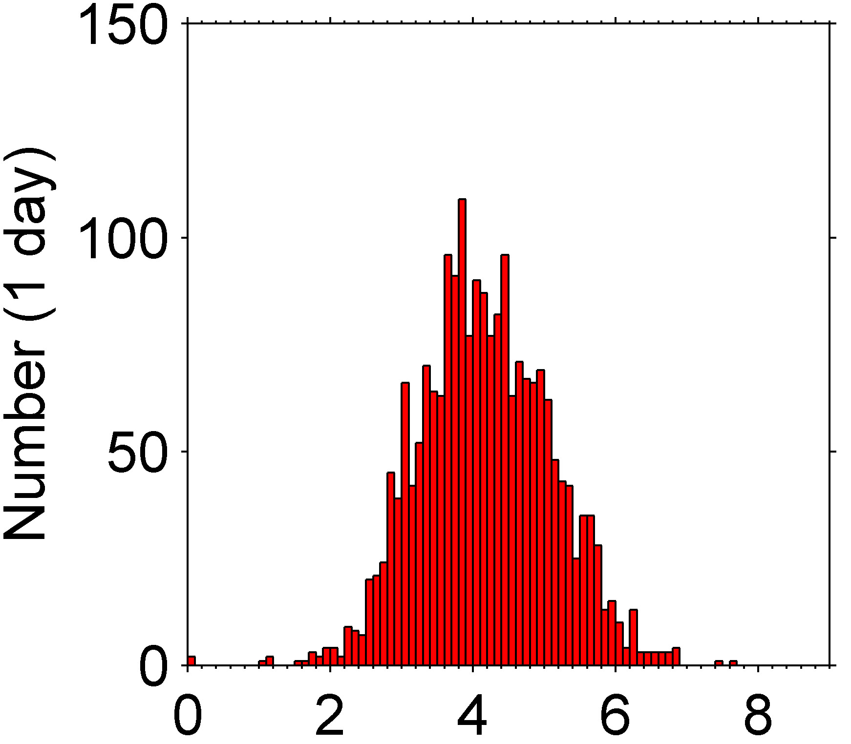
- First, we calculate a magnitude histogram to get a better sense of the data.
- Next, we calculate the magnitude of completeness (Mc). Remove the mainshock from the dataset. You may wish to both temporally, and spatially filter the data as well.
- There are several different methods for calculating the Mc. We will focus on 3.
- Maximum curvature: finds the point where the non-cumulative distribution (histogram) has the highest curvature.
- Goodness of fit (90%,95%): compares observed FMD with synthetics on a per bin basis. Residual determines the goodness of fit. ZMAP defaults to MAXC if it is not available.
- Entire magnitude range: uses a model which fits the entire data range by using a G-R for the complete part and and cumulative normal distribution for the incomplete part of the non cumulative FMD. Basically, fits all of the data.
- In MATLAB, we can use the following function.
-
nMethod =1; % MAX CURVE OR nMethod=5; % BEST COMBINATION OR nMethod=6; % EMR
fBinning = 0.1; % size of our magnitude bins
fMcCorrection = .2; % Used to add a correction because maximum curvature often underestimates Mc
[fMc] = calc_Mc(mCatalog, nMethod, fBinning, fMcCorrection);
- This will yield a tenative estimate of the Mc. We now need to determine the associated b-value. We will focus on 2 methods, the maximum liklihood method and a least squares fit. ZMAP uses the maximum liklihood method.
- Before estimating the b-value, data below the Mc should be removed. Keep data at and above the Mc. The mainshock should be removed as well.
% BIN is the binsize (.1) and magVec is the vector of magnitudes at and above the Mc
% b is the bvalue, a is the a-value, and std_err is the error/li>
[b, a, std_err] = bval_lsqreg(magVec, bin); % LEAST SQUARES
[b1, a1, std_err1] = bval_maxlkh2(magVec, bin); % Maximum Liklihood
If we plot the 2 methods against the # of events left at each Mc, we get a plot like this:
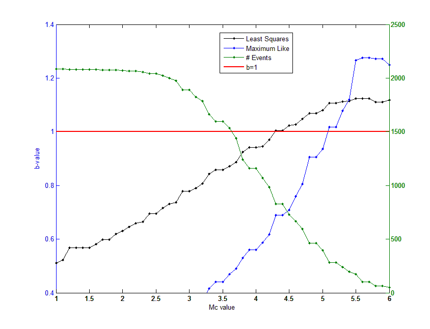 Remember that these are estimates and you may find that different methods yield a different Mc. A small variation between them, such as 4.8,4.9,5.0 is usually not important.
In this case, one can choose 5.0 since the # of events at 4.8 is not likely to be much greater. If you know the data is reasonably magnitude complete, then the associated b-value should be close to ~1
, perhaps in the range 0.9-1.1, since the error is usually ~10% anyways. However, if your results yield 3.6, 4.0, 4.6, you will need to closely inspect both
the b-value variation with Mc and the histogram since it is likely that your data is either incomplete, or is including aftershocks from other events.
Remember that these are estimates and you may find that different methods yield a different Mc. A small variation between them, such as 4.8,4.9,5.0 is usually not important.
In this case, one can choose 5.0 since the # of events at 4.8 is not likely to be much greater. If you know the data is reasonably magnitude complete, then the associated b-value should be close to ~1
, perhaps in the range 0.9-1.1, since the error is usually ~10% anyways. However, if your results yield 3.6, 4.0, 4.6, you will need to closely inspect both
the b-value variation with Mc and the histogram since it is likely that your data is either incomplete, or is including aftershocks from other events.
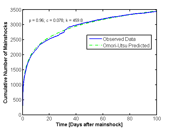
Part 2: The Modified Omori Law
- We will use the script f_calc_omori_auto to calculate the MOL parameters. Note, you will need to pass in the mainshock.
-
windowInDays=100;
bootstraps=300;
model=1;
evt_time=mtx_tempcatalog(1:end,11);
evt_mag=mtx_tempcatalog(1:end,6);
blankfigurehandle=figure;
[p,k,c,timevec,winsize,time_as,cummodel,cumobs,ksstuff,fAIC,fRMS,nMod,mRes]= f_calc_omori_auto(windowInDays,bootstraps,model,evt_time,evt_mag,blankfigurehandle);
-
- Great in-depth introductions to all of the below topics can be found at the Community Online Resource for Statistical Seismicity Analysis
- Mc estimation
- Woessner, J., J. Hardebeck, and E. Hauksson (2010), What is an instrumental seismicity
catalog?, in Understanding Seismicity Catalogs and their Problems, pp. 1–14.
- Woessner, J., and S. Wiemer (2005), Assessing the Quality of Earthquake Catalogues:
Estimating the Magnitude of Completeness and Its Uncertainty, Bulletin of the
Seismological Society of America, 95(2), 684–698, doi:10.1785/0120040007.
- Wiemer, S., and M. Wyss (2000), Minimum Magnitude of Completeness in Earthquake
Catalogs: Examples from Alaska, the Western United States, and Japan, Bulletin of the
Seismological Society of America, 90(4), 859–869, doi:10.1785/0119990114.
- G-R and b-value
- Marzocchi, W., and L. Sandri (2003), A review and new insights on the estimation of the b-
value and its uncertainty, Annals of geophysics, 46(December).
- Boettcher, M. S., a. McGarr, and M. Johnston (2009), Extension of Gutenberg-Richter
distribution to M W -1.3, no lower limit in sight, Geophysical Research Letters, 36(10), 1–
5, doi:10.1029/2009GL038080.
- Frohlich, C., and S. D. Davis (1993), Teleseismic b Values; Or, Much Ado About 1.0, Journal
of Geophysical Research, 98(B1), 631–644, doi:10.1029/92JB01891.
- Okal, E. A., and B. A. Romanowicz (1994), On the variation of b-values with earthquake s ize,
Physics of the Earth and Planetary Interiors, 87(1-2), 55–76, doi:10.1016/0031-
9201(94)90021-3.
- Modified Omori Law and p-values
- Nyffenegger, P., and C. Frohlich (1998), Recommendations for Determining p Values for
Aflershock Sequences and Catalogs, Bulletin of the Seismological Society of America,
88(5), 1144–1154.
- Utsu, T., Y. Ogata, and R. Matsu’ura (1995), The centenary of the Omori formula for a decay
law of aftershock activity, Journal of Physics of the Earth, 43(1), 1–33.
- Utsu, T. (1961), A statistical study of the occurrence of aftershocks, Geophysical Magazine, 30,
521–605.
- Tosi, P., V. Rubeis, and P. Sbarra (2010), Stacked Analysis of Earthquake Sequences:
Statistical Space–Time Definition of Clustering and Omori Law Behavior, in
Synchronization and Triggering: from Fracture to Earthquake Processes, vol. 1, edited by
V. Rubeis, Z. Czechowski, and R. Teisseyre, pp. 323–337, Springer Berlin Heidelberg.
- Omori, F. (1894), On the after-shocks of earthquakes, Journal of the College of Science,
Imperial University of Tokyo, 7, 111-200.
- Aftershock rate estimation
- van Stiphout, T., D. Schorlemmer, and S. Wiemer (2011), The Effect of Uncertainties on
Estimates of Background Seismicity Rate, Bulletin of the Seismological Society of
America, 101(2), 482–494, doi:10.1785/0120090143.
- Synthetic aftershocks
- Felzer, K. R. (2012), Stochastic ETAS Aftershock Simulator Program,
http://pasadena.wr.usgs.gov/office/kfelzer/AftSimulator.html.
- Felzer, K. R., T. W. Becker, R. E. Abercrombie, G. Ekstrom, and J. R. Rice (2002), Triggering
of the 1999 M W 7.1 Hector Mine earthquake by aftershocks of the 1992 M W 7.3 Landers
earthquake, Journal of Geophysical Research, 107(B9), 1–13, doi:10.1029/2001JB000911.
- Ogata, Y. (1998), Space-Time Point-Process Models for Earthquake Occurrences, Annals of the
Institute of Statistical Mathematics, 50(2), 379–402, doi:10.1023/A:1003403601725.
- Ogata, Y. (1988), Statistical models for earthquake occurrences and residual analysis for point
processes, Journal of the American Statistical Association, 83(401), 9–27.
|