Once a cpt file has been made it is relatively straightforward to generate a color image of a gridded data. Here, we will extract a subset of the global 30" DEM (data id 9) from USGS:
grdraster 9 -R-108/-103/35/40 -Gus.grd
Using grdinfo we find that the data ranges from ![]() 1000m to
1000m to
![]() 4300m so we make a cpt file accordingly:
4300m so we make a cpt file accordingly:
makecpt -Crainbow -T1000/5000/500 -Z >! topo.cpt
Color images are made with grdimage which takes the usual common command options (by default the -R is taken from the data set) and a cptfile; the main other options are
We want to make a plain color map with a color bar superimposed above the plot. We try
grdimage us.grd -JM6i -P -B2 -Ctopo.cpt -V -K >! topo.ps
psscale -D3i/8.5i/5i/0.25ih -Ctopo.cpt -I0.4 -B/:m: -O >> topo.ps
The plain color map lacks detail and fails to reveal the topographic
complexity of this Rocky Mountain region. What it needs is artificial
illumination. We want to simulate shading by a sun source in the east,
hence we derive the required intensities from the gradients of the
topography in the N90![]() E direction using grdgradient. Other than the
required input and output filenames, the available options are
E direction using grdgradient. Other than the
required input and output filenames, the available options are
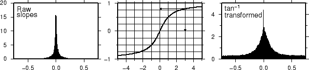
Figure 4.1 shows that raw slopes from bathymetry tend to be
far from normally distributed (left). By using the inverse tangent
transformation we can ensure a more uniform distribution (right).
The inverse tangent transform simply takes the raw slope estimate
(the x value at the arrow) and returns the corresponding inverse
tangent value (normalized to fall in the ![]() range; horizontal
arrow pointing to the y-value).
range; horizontal
arrow pointing to the y-value).
Both -Ne and -Nt yield well behaved gradients. Personally, we prefer to use the -Ne option; the value of norm is subjective and you may experiment somewhat in the 0.5-5 range. For our case we choose
grdgradient us.grd -Ne0.8 -A100 -M -Gus_i.grd
Given the cpt file and the two gridded data sets we can create the shaded relief image:
grdimage us.grd -Ius_i.grd -JM6i -P -B2 -Ctopo.cpt -K >! topo.ps
psscale -D3i/8.5i/5i/0.25ih -Ctopo.cpt -I0.4 -B/:m: -O >> topo.ps