This transformation converts polar coordinates (angle ![]() and radius
and radius ![]() )
to positions on a plot. Now
)
to positions on a plot. Now
![]() and
and
![]() , hence it is similar
to a regular map projection because
, hence it is similar
to a regular map projection because ![]() and
and ![]() are coupled and
are coupled and ![]() (i.e.,
(i.e., ![]() ) has a 360
) has a 360![]() periodicity.
With input and output points both in the plane it is a two-dimensional projection.
The transformation comes in two flavors:
periodicity.
With input and output points both in the plane it is a two-dimensional projection.
The transformation comes in two flavors:
Consequently, the polar transformation is defined by providing
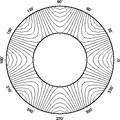
As an example of this projection we will create a gridded data set
in polar coordinates
![]() using grdmath, a RPN calculator that operates on or
creates grdfiles.
using grdmath, a RPN calculator that operates on or
creates grdfiles.
grdmath -R0/360/2/4 -I6/0.1 X 4 MUL PI MUL 180 DIV COS Y 2 POW MUL = test.grd
grdcontour test.grd -JP3i -B30Ns -P -C2 -S4 --PLOT_DEGREE_FORMAT=+ddd > GMT_polar.ps
rm -f test.grd
We used grdcontour to make a contour map of this data. Because
the data file only contains values with
![]() , a donut
shaped plot appears in Figure 5.6.
, a donut
shaped plot appears in Figure 5.6.