The GMT programs filter1d (for tables of data indexed
to one independent variable) and grdfilter (for data
given as 2-dimensional grids) allow filtering of data by a
moving-window process. (To filter a grid by Fourier transform use
grdfft.) Both programs use an argument
-F![]() type
type![]() width
width![]() to specify the type of
process and the window's width (in 1-d) or diameter (in 2-d).
(In filter1d the width is a length of the time or
space ordinate axis, while in grdfilter it is the
diameter of a circular area whose distance unit is related to
the grid mesh via the -D option). If the process is a
median, mode, or extreme value estimator then the window
output cannot be written as a convolution and the filtering
operation is not a linear operator. If the process is a weighted
average, as in the boxcar, cosine, and gaussian filter types,
then linear operator theory applies to the filtering process.
These three filters can be described as convolutions with an
impulse response function, and their transfer functions
can be used to describe how they alter components in the input
as a function of wavelength.
to specify the type of
process and the window's width (in 1-d) or diameter (in 2-d).
(In filter1d the width is a length of the time or
space ordinate axis, while in grdfilter it is the
diameter of a circular area whose distance unit is related to
the grid mesh via the -D option). If the process is a
median, mode, or extreme value estimator then the window
output cannot be written as a convolution and the filtering
operation is not a linear operator. If the process is a weighted
average, as in the boxcar, cosine, and gaussian filter types,
then linear operator theory applies to the filtering process.
These three filters can be described as convolutions with an
impulse response function, and their transfer functions
can be used to describe how they alter components in the input
as a function of wavelength.
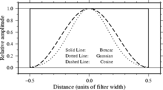
Impulse responses are shown here for the boxcar, cosine, and gaussian filters. Only the relative amplitudes of the filter weights shown; the values in the center of the window have been fixed equal to 1 for ease of plotting. In this way the same graph can serve to illustrate both the 1-d and 2-d impulse responses; in the 2-d case this plot is a diametrical cross-section through the filter weights (Figure J.1).
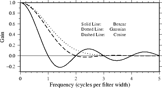
Although the impulse responses look the same in 1-d and 2-d,
this is not true of the transfer functions; in 1-d the transfer
function is the Fourier transform of the impulse response,
while in 2-d it is the Hankel transform of the impulse response.
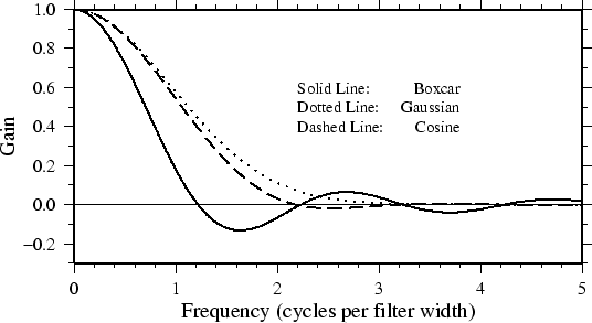
These are shown in Figures J.2 and
J.3, respectively. Note that in 1-d the boxcar transfer
function has its first zero crossing at ![]() , while in 2-d
it is around
, while in 2-d
it is around ![]() . The 1-d cosine transfer function
has its first zero crossing at
. The 1-d cosine transfer function
has its first zero crossing at ![]() ; so a cosine filter needs
to be twice as wide as a boxcar filter in order to zero the same
lowest frequency. As a general rule, the cosine and gaussian
filters are ``better'' in the sense that they do not have the
``side lobes'' (large-amplitude oscillations in the transfer
function) that the boxcar filter has. However, they are
correspondingly ``worse'' in the sense that they require more
work (doubling the width to achieve the same cut-off wavelength).
; so a cosine filter needs
to be twice as wide as a boxcar filter in order to zero the same
lowest frequency. As a general rule, the cosine and gaussian
filters are ``better'' in the sense that they do not have the
``side lobes'' (large-amplitude oscillations in the transfer
function) that the boxcar filter has. However, they are
correspondingly ``worse'' in the sense that they require more
work (doubling the width to achieve the same cut-off wavelength).
One of the nice things about the gaussian filter is that its
transfer functions are the same in 1-d and 2-d. Another nice
property is that it has no negative side lobes. There are many
definitions of the gaussian filter in the literature (see page
7 of BracewellJ.1). We
define ![]() equal to 1/6 of the filter width, and the impulse
response proportional to
equal to 1/6 of the filter width, and the impulse
response proportional to
![]() . With this
definition, the transfer function is
. With this
definition, the transfer function is
![]() and the wavelength at which the transfer function equals 0.5 is
about 5.34
and the wavelength at which the transfer function equals 0.5 is
about 5.34 ![]() , or about 0.89 of the filter width.
, or about 0.89 of the filter width.