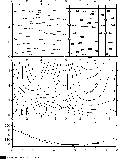
This example shows how one goes from randomly spaced data points to an evenly sampled surface. First we plot the distribution and values of our raw data set (table 5.11 from example 12). We choose an equidistant grid and run blockmean which preprocesses the data to avoid aliasing. The dashed lines indicate the logical blocks used by blockmean; all points inside a given bin will be averaged. The logical blocks are drawn from a temporary file we make on the fly within the shell script. The processed data is then gridded with the surface program and contoured every 25 units. A most important point here is that blockmean, blockmedian, or blockmode should always be run prior to running surface, and both of these steps must use the same grid interval. We use grdtrend to fit a bicubic trend surface to the gridded data, contour it as well, and sample both gridded files along a diagonal transect using grdtrack. The bottom panel compares the gridded (solid line) and bicubic trend (dashed line) along the transect using psxy (Figure 7.14):
#!/bin/csh
#        GMT EXAMPLE 14
#
#        $Id: job14.csh,v 1.8 2004/06/02 22:52:32 pwessel Exp $
#
# Purpose:    Showing simple gridding, contouring, and resampling along tracks
# GMT progs:    blockmean, grdcontour, grdtrack, grdtrend, minmax, project
#        pstext, psbasemap, psxy, surface
# Unix progs:    $AWK, rm
#
# First draw network and label the nodes
gmtset GRID_PEN_PRIMARY 0.25p,-
psxy table_5.11 -R0/7/0/7 -JX3.06i/3.15i -B2f1WSNe -Sc0.05i -Gblack -P -K -Y6.45i >! example_14.ps
$AWK '{printf "%g %s 6 0 0 LM %g\n", $1+0.08, $2, $3}' table_5.11 | pstext -R -J -O -K -N \
   >> example_14.ps
blockmean table_5.11 -R0/7/0/7 -I1 >! mean.xyz
# Then draw blockmean cells
psbasemap -R0.5/7.5/0.5/7.5 -J -O -K -B0g1 -X3.25i >> example_14.ps
psxy -R0/7/0/7 -J -B2f1eSNw mean.xyz -Ss0.05i -Gblack -O -K >> example_14.ps
$AWK '{printf "%g %s 6 0 0 LM %g\n", $1+0.1, $2, $3}' mean.xyz | pstext -R -J -O -K -W255o \
   -C0.01i/0.01i -N >> example_14.ps
# Then surface and contour the data
surface mean.xyz -R -I1 -Gdata.grd
grdcontour data.grd -J -B2f1WSne -C25 -A50 -G3i/10 -S4 -O -K -X-3.25i -Y-3.55i >> example_14.ps
psxy -R -J mean.xyz -Ss0.05i -Gblack -O -K >> example_14.ps
# Fit bicubic trend to data and compare to gridded surface
grdtrend data.grd -N10 -Ttrend.grd
project -C0/0 -E7/7 -G0.1 > track
grdcontour trend.grd -J -B2f1wSne -C25 -A50 -Glct/cb -S4 -O -K -X3.25i >> example_14.ps
psxy -R -J track -W1pto -O -K >> example_14.ps
# Sample along diagonal
grdtrack track -Gdata.grd | cut -f3,4 >! data.d
grdtrack track -Gtrend.grd | cut -f3,4 >! trend.d
psxy `minmax data.d trend.d -I0.5/25` -JX6.3i/1.4i data.d -W1p -O -K -X-3.25i -Y-1.9i -B1/50WSne \
   >> example_14.ps
psxy -R -J trend.d -W0.5pta -O -U"Example 14 in Cookbook" >> example_14.ps
\rm mean.xyz track *.grd *.d .gmt*