As our second example we will demonstrate how to make color
images from gridded data sets (again, we will deferr the
actual making of gridded files to later examples). We will
use the supplemental program grdraster to extract 2-D
grdfiles of bathymetry and Geosat geoid heights and put the
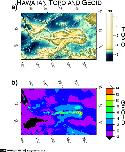
two images on the same page. The region of interest is the
Hawaiian islands, and due to the oblique trend of the island
chain we prefer to rotate our geographical data sets using
an oblique Mercator projection defined by the hotspot pole
at (68![]() W, 69
W, 69![]() N). We choose the point (190
N). We choose the point (190![]() ,
25.5
,
25.5![]() ) to be the center of our projection (e.g., the
local origin), and we want to image a rectangular region
defined by the longitudes and latitudes of the lower left
and upper right corner of region. In our case we choose
(160
) to be the center of our projection (e.g., the
local origin), and we want to image a rectangular region
defined by the longitudes and latitudes of the lower left
and upper right corner of region. In our case we choose
(160![]() , 20
, 20![]() ) and (220
) and (220![]() , 30
, 30![]() ) as the
corners. We use grdimage to make the illustration:
) as the
corners. We use grdimage to make the illustration:
#!/bin/csh
#        GMT EXAMPLE 02
#
#        $Id: job02.csh,v 1.9 2006/03/06 09:43:48 pwessel Exp $
#
# Purpose:    Make two color images based gridded data
# GMT progs:    gmtset, grd2cpt, grdgradient, grdimage, makecpt, psscale, pstext
# Unix progs:    cat rm
#
gmtset HEADER_FONT_SIZE 30 OBLIQUE_ANNOTATION 0
#get gridded data using GMT supplemental program grdraster
#grdraster 1 -R160/20/220/30r -JOc190/25.5/292/69/4.5i -GHI_topo2.grd=0/0.001/0
#grdraster 4 -R -JO -GHI_geoid2.grd
makecpt -Crainbow -T-2/14/2 >! g.cpt
grdimage HI_geoid2.grd -R160/20/220/30r -JOc190/25.5/292/69/4.5i -E50 -K -P -B10 -Cg.cpt \
   -U/-1.25i/-1i/"Example 2 in Cookbook" -X1.5i -Y1.25i >! example_02.ps
psscale -Cg.cpt -D5.1i/1.35i/2.88i/0.4i -O -K -L -B2:GEOID:/:m: -E >> example_02.ps
grd2cpt HI_topo2.grd -Crelief -Z >! t.cpt
grdgradient HI_topo2.grd -A0 -Nt -GHI_topo2_int.grd
grdimage HI_topo2.grd -IHI_topo2_int.grd -R -J -E50 -B10:."H@#awaiian@# T@#opo and @#G@#eoid:" \
   -O -K -Ct.cpt -Y4.5i >> example_02.ps
psscale -Ct.cpt -D5.1i/1.35i/2.88i/0.4i -O -K -I0.3 -B2:TOPO:/:km: >> example_02.ps
cat << EOF | pstext -R0/8.5/0/11 -Jx1i -O -N -Y-4.5i >> example_02.ps
-0.4 7.5 30 0.0 1 CB a)
-0.4 3.0 30 0.0 1 CB b)
EOF
\rm -f .gmtcommands4 .gmtdefaults4 HI_topo2_int.grd ?.cpt
The first step extracts the 2-D data sets from the local data base using grdraster, which is a supplemental utility program (see Appendix A) that may be adapted to reflect the nature of your data base format. It automatically figures out the required extent of the region given the two corners points and the projection. The extreme meridians and parallels enclosing the oblique region is -R159:50/220:10/3:10/47:35. This is the area extracted by grdraster. For your convenience we have commented out those lines and provided the two extracted files so you do not need grdraster to try this example. By using the embedded grdfile format mechanism we saved the topography using kilometers as the data unit. We now have two grdfiles with bathymetry and geoid heights, respectively. We use makecpt to generate a linear color palette file geoid.cpt for the geoid and use grd2cpt to get a histogram-equalized cpt file topo.cpt for the topography data. To emphasize the structures in the data we calculate the slopes in the north-south direction using grdgradient; these will be used to modulate the color image. Next we run grdimage to create a color-code image of the Geosat geoid heights, and draw a color scale to the right of the image with psscale. We also annotate the color scales with psscale. Similarly, we run grdimage but specify -Y4.5i to plot above the previous image. Adding scale and label the two plots a) and b) completes the illustration (Figure 7.2).