Dislocation Modeling using GTdef for Modern Geodetic Methods

GTdef is an implementation of the Okada (1985) dislocation model written by Ting Chen and Lujia Feng, with codes modified from disl written by Peter Cervelli. Okada (1985) can describe the surface deformation associated with rectangular dislocations of arbitrary orientation within a purely-elastic, isotropic, poisson-solid, half-space. Dislocations can be described by either dip-slip, strike-slip, or opening, and hence can be used to describe a range of processes including earthquake faulting, interseismic coupling, and planar fluid changes like magmatic dike inflation or groundwater withdrawal.

The code here is developed so that one could perform both forward models that predict ground deformation and inverse models that use data with errors and some modeling constraints to predict information about the source. The source in either case can be either simple rectangular slips along the plane, orthogonal to it or some combination of both. Here, we'll step through first some forward models, and eventually inversions. However, here, we will only focus on Forward Models; meaning that we will perscribe a fault with a certain deformational character to it, and then observe the output deformational field.

Starting Notes:

• Matlab: Algorithms are written in Matlab and require the 'Parameter estimation' toolbox for inversions.
• Matlab Path: The programs currently work on our internal Linux network. Be sure to add the program path to your start-up file for Matlab to ensure you can use the program in the future.

   % mkdir ~/matlab
   % echo "path('/home/lfeng/DEF/GTdef',path);" >> ~/matlab/startup.m 

• Current Version: Right now we are working with GTdef version 1.5. Lujia is currently working on an implementation that will allow for layered elastic geometries.

Performing models:

1. Input File: This is the only documentation other than within the code, and this webpage (which is in development). As you will be able to see there are a number of ways to both describe the input 'fault' models, as well as output data.
2. Simple Planar Forward Models :
   1. Strike-Slip Faults: Create a 45 km long vertical (90° dip) planar fault, with 1 meter of right-lateral strike-slip motion, and slipping to 15 km depth.
      • Create input file:
        For the output, we will describe the spatial deformation every 2 km across a 60x60 km grid surrounding the deformation.
        

         % echo "
           coord local
           fault 2 MySSFault 0 -22.5e3 0 22.5e3 0e3 15e3 90 -1 0 0  0 0  0 0  0 0
           grid 2kmx2km 0 0 -30e3 -30e3 30e3 30e3 16 16 " > local1.in
         

        
        
      • Run GTdef

         # within matlab
         > GTdef('local1.in',1) % the '1' is for one core  
        

        
        This will create an output file called 'local1_fwd.out'
        
      • Now visualize the output using gnuplot to show the full vector field.

        % gnuplot
         gnuplot>  set size square
         gnuplot>  set view 60,30,1,.33
         gnuplot>  splot '< egrep "point 3" local1_fwd.out' u 4:5:(0):($7*1e4):($8*1e4):($9*1e4) w vect ,\
          "< egrep MySSFault local1_fwd.out | awk '{print $4,$5,-$8}{print $6,$7,-$8}{print $6,$7,-$9}{print $4,$5,-$9}{print $4,$5,-$8}' " w l lt -1 
          % use the cursor to move around the data
        

        
        
   2. Low-Angle Thrust Fault: Create a 200 km long vertical (30° dipping) planar thrust fault, with 5 meter of thrust motion. The down-dip fault width should be 100 km.
      • Create input file:
        Note that you can experiment with each:
        1. the method you're using to characterize your input fault
        2. the output solutions (grid, profile, individual points)
        3. you may even want to try this in geographic coordinates, and perform the proper calculations to put this along a real subduciton zone.
        4. After you've created and ran this model, you may want to try one with a component of strike-slip motion, as well, as a more complicated fault.

           Be sure to name your input file differently than your original.
         % # if you know how, you can create the input file directly within an editor (e.g. vim)
         		

        
        
      • Run GTdef

         # within matlab
        

        
        This will create an new output file.
        
      • Now visualize the output using the software of your choice (e.g. matlab, GMT, gnuplot, even....excel!)
        
        
      
      
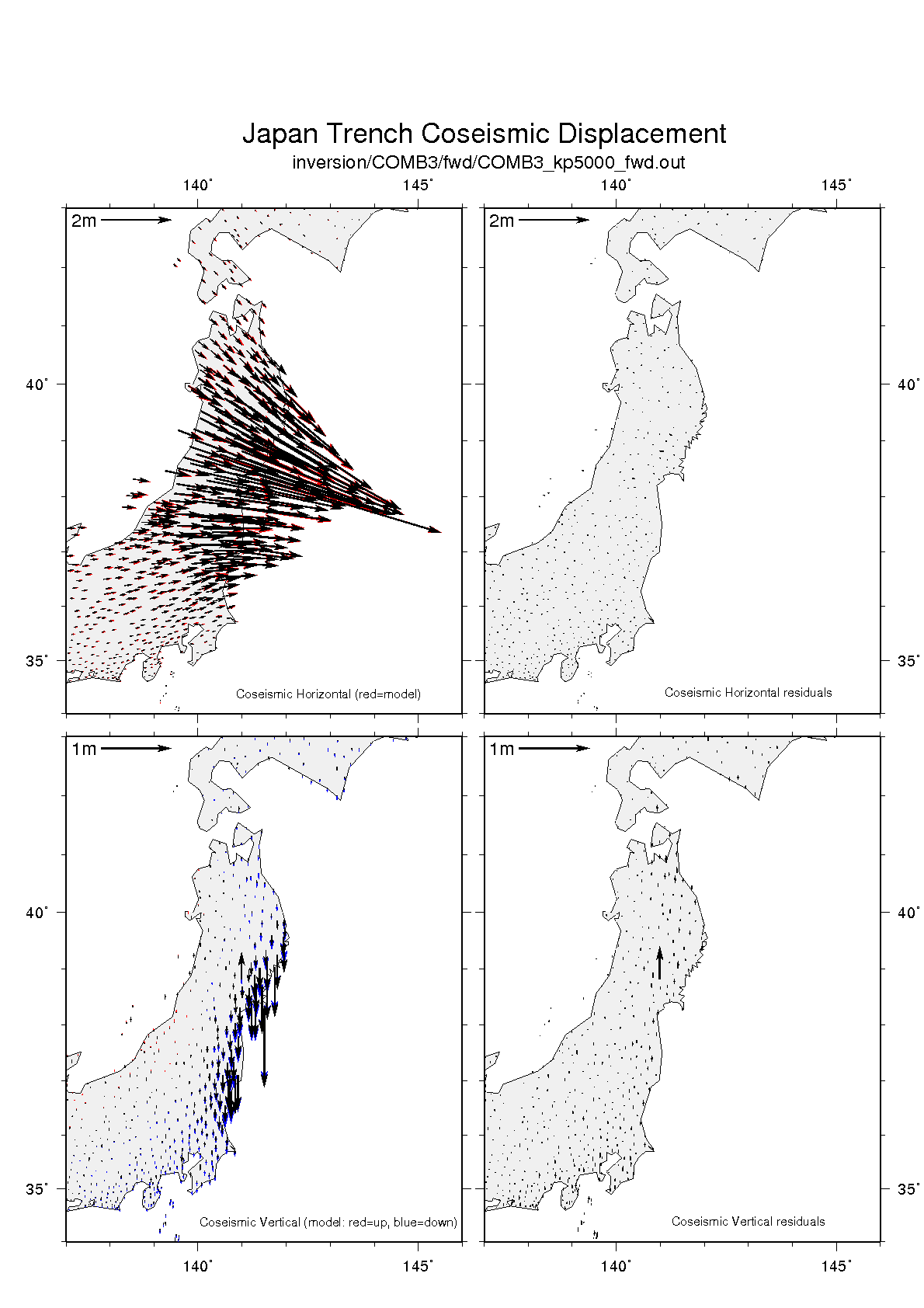
   3. Another low-Angle Thrust Fault: Here is an example of a model solution that we generated for the 2011 Tohoku-Oki Earthquake using both GPS onland and tsunami wave predictions for seafloor displacement. This was created from an inversion of 128 sub-patches, each allowing for both dip-slip, and transvese motions.
      Here is a simple illustration showing the displacement field along the thrust (model is removed from the geographic projection).
      Here is a comparison between the lateral and vertical GPS field with the earthquake rupture model.